Link to Cubic Spline Update
The previous two posts used cubic splines with the “natural” end condition, that is with an end curvature of zero. To apply the cubic spline to analysis of continuous beams with different end conditions we need to find the cubic spline formulation for a specified non-zero end curvature, or for a specified slope.
To that end, I have re-written the CSpline function to show more explicitly the parameters of the underlying cubic equations, and how these relate to the chosen end conditions. The new function and examples can be found at CSpline2.zip. The procedure is as follows:
Aim: For a list of XY coordinates, X(1 to n) and Y(1 to n), to find a, b, c, d in
Y = a + b(x – X(i)) + c(x – X(i))^2 + d(x- X(i))^3
for each segment, where x lies between X(i) and X(i+1)
It can be shown that:
a = Y(i)
b = m(i) – l(i)/6(2c(i) + c(i+1))
c = c(i)/2
d = (c(i+1) – c(i)) / (6l(i))
where:
l(i) = x(i+1) – x(i)
m(i) = (y(i+1) – y(i)) / l(i)
c(i) = d2y/dx2 at point i
The values of l and m are defined by the x,y coordinates, so it remains to find the values of c .
Since m and c (the first and second derivative of f(x)) are defined to be equal for the splines meeting at any node
it can be shown that for any point, i:
l(i-1)c(i-1) + 2(l(i-1) + l(i))c(i) + l(i)(c(i+1)) = 6(m(i) – m(i-1))
In matrix form:
 A spline with n segments will have n+1 nodes and n-1 internal nodes, so 2 more equations are required to define the c values
Commonly used end conditions include:
Specified second derivative. Where the second derivative = 0 the spline is known as a natural spline.
Specified first derivative. This is known as a clamped spline.
Examples of the equations for different end conditions, and their solution using worksheet functions, are given on the spreadsheet. On the spreadsheet the matrix equations are solved using the built-in MINVERSE() and MMULT() functions, but for the CSplineA UDF it is much more efficient to use a specific routine for solving “tri-diagonal” matrices, i.e. those where the only non-zero terms are on or immediately adjacent to the leading diagonal.
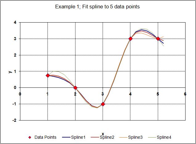
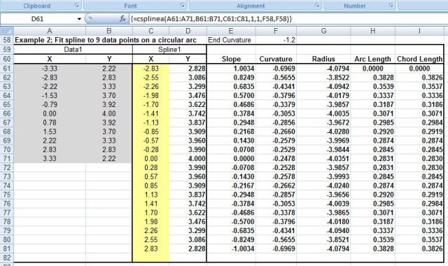
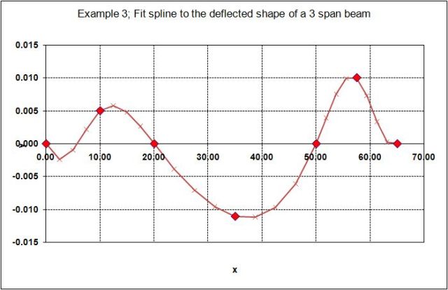
Examples of the use of the new function, with different end conditions, are shown below:


I did quite a bit of analysis on this a while ago and found that the “smooth curve” option on an xy plot matches closely enough for many practical purposes and also that a clamped spline could be simulated by adding an extra point at each end. Worksheet formulas and further info can be found on the charting newsgroup. All cubic splines only approximate the “true” shape that minimises curvature in the xy plane.
To see the connection, one can look at the derivative matrix D(i,j) as in eqn (18): http://mathworld.wolfram.com/CubicSpline.html
– For a basic approximation we can combine the off diagonal entries to get 6’s along the interior main diagonal entries. Inverting this then reduces to the basic Excel curve (cardinal spline with tension 0.5).
– For larger samples the inverse of the tridiagonal matrix tends to: (√3-2)^|i-j| /(2√3) at interior points (which agrees closely with MINVERSE.) From this we can see the natural spline is generally less tight (eg tension = √3/2 in the symmetric case).
LikeLike
Hi Lori – thanks for the interesting comments and links.
You said “All cubic splines only approximate the “true” shape that minimises curvature in the xy plane. ”
Which is true, as can be seen from the approximation to a circular arc in one of the examples, but what makes the formulation of the cubic spline particularly interesting to me, as an engineer, is that the approximation is exactly the same approximation as that embodied in the Euler-Bernoulli theory of beam bending. This means we can use a cubic spline analysis to derive bending moments and shear forces in a beam, and get exact agreement, of forces and deflections, with the output from a finite element analysis program, using beam elements.
LikeLike
Thanks for the explanation, that makes sense. The cubic spline is an elegant model and, as i understand it, exactly solves the linearised problem for small deflections without stiffness. Euler apparently spent many years on the underlying problem: http://levien.com/phd/euler_hist.pdf
I’m no engineer but it seems that the Euler-Bernoulli theory is flexible from the point of view of functional form so perhaps other formulations might be useful for comparison too eg which incorporate tension: http://msdn.microsoft.com/en-us/library/ms536358(VS.85).aspx. A simple calculation seemed to produce some similar results although the curvature was not continuous at the joins.
LikeLike
Excellent work, I could have done with this about 7 years ago when I was at uni!
LikeLike
Pingback: Continuous beam with specified end conditions … « Newton Excel Bach, not (just) an Excel Blog
Both dougaj4 & Lori’s work is excellent – many copies of your posts circulating on various websites.
Just one query, is it possible to use a cubic spline (or Catmull-Rom or Bezier) function on a unsorted Excel data set?
This is continuing the “How to get the corresponding X value for a given Y value?” question posed by others – to which Lori submitted a great Catmull-Rom solution using standard Excel worksheet functions (http://help.lockergnome.com/office/default–ftopict1005590.html).
However on exchanging X and Y data the interpolation will fail at particular values because the original Y data (now X for interpolation) is not sorted in ascending order. This issue is not corrected if the original data is sorted for ascending Y before exchanging sets and interpolating.
It seems that all the interpolation solutions I’ve come across, rely on the X data being in ascending order. Is there a way to get around this?
LikeLike
Charlie – The relevant part of the formula from that post is: MATCH(D4,A4:A14,-1)-2
This locates the interval of interest in a descending data set, if data is ascending just use +1 for the last argument for each instance within the formula.
For a more general solution try: MATCH(A4=D4,0)-3
This locates the first interval containing the chosen point and applies to unordered data (with points consecutively plotted) although there may be more than one corresponding value so the result may not be well-defined.
Similar considerations apply to other interpolation formulas.
(Note: in the second example it should have been y=50 not y=0.5)
Doug – i appreciate your making this specialist knowledge freely available. These posts are very informative and I’ve been following the continued development with great interest and look forward to further posts on this topic.
LikeLike
forgot about HTML tags – trying second formula again:
MATCH(A4<=D4,A4:A14>=D4,0)-3
LikeLike
Charlie – I hope Lori’s replies gave you what you want. I may well be looking at this in more detail later, but for the time being I’m concentrating on applying this to the analysis of straight beams, so the requirement for ascending X is not an issue.
You might also like to investigate the application of bezier curves to defining typographical fonts, which have to deal with ascending and descending x values.
LikeLike
Pingback: Cubic Spline Update « Newton Excel Bach, not (just) an Excel Blog